|
Overview
The objective of NARCCAP Experiment 0 is to examine the possible influence of regional climate model domain size and boundary location on simulated meteorological fields in the domain interior. Previous experiments have suggested that regional climate model domains that are too large may allow the climate simulated by the regional model to decouple unrealistically from that of the driving boundary conditions. In contrast, if the domain is too small, the regional model may not have sufficient physical space to fully develop the dominant mesoscale flow features indigenous to the region. Also, if the domain is not optimally located it may not allow for sufficient horizontal space for coupling to remote large-scale forcing features.
Experimental Design
The Regional Climate Modeling Laboratory at Iowa State University will manage
Experiment 0. The modeling team will perform a series of 1-year simulations with alternative domains and with boundary conditions supplied by the NCEP/DOE Reanalysis - II (R2) data. Land/ocean distribution and preferred flow directions for meteorological systems suggest that the direction of domain enlargement might make a difference. To allow for this possibility, a series of up to four simulations will be performed, as described below. Each group should perform at least the first two. Each run will consist of a 12-month simulation beginning January 1979.
Base Computational Domain
| Number of points in the x-direction: | 155 |
| Number of points in the y-direction: | 130 |
| Horizontal grid spacing in kilometers: | 50 |
| Center latitude location: | 47.5 |
| Center longitude location: | -97 |
| Equator latitude location: | 47.5 |
| Equator longitude location: | -97 |
| Map projection: | Rotated Mercator |
Note that a Lambert conformal conical projection true at 30N and 60N will give a similar domain.
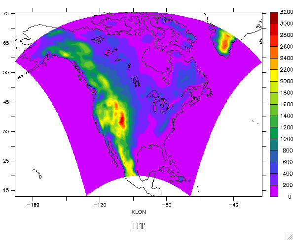
The base computational domain with orography is given in Figure 1.
 | |
Figure 1. Computational domain for base case for NARCCAP Experiment 0. |
Driving Data Fields
Reanalysis data
Driving fields for Experiment 0 are supplied by the NCEP/DOE Reanalysis - II (R2) data. Each modeling group should access the R2 data directly from one of the three sources given below depending on which is more convenient. Each year of R2 data is over 3 GB, so make sure you have enough free disk space before you do the transfer.
Sources
- Web links to the R2 (and other reanalysis) archives are supplied on the RegCM3 home page at the International Center for Theoretical Physics (ICTP). These links point to the archive of 2.5x2.5 lat/lon pressure-level output stored at the NOAA Climate Diagnostics Center (CDC). The files are in netCDF format.
- The data also may be acquired directly from the NCAR Mass Storage System where it is stored in GRIB format (a convenience for those using MM5 or others that already have GRIB decoders for these data). See
http://dss.ucar.edu/datasets/ds091.0
- A third source of the data is a mirror site of the NCAR Mass Storage System R2 archive established by the ISU RCM Lab. The mirror site contains only the R2 data needed to drive RCMs. It is accessed through the following URL:
http://pircsds0.agron.iastate.edu/pircs1c
Sea Surface Temperature and Sea Ice
Considerations when selecting a source for sea surface temperature (SST) and sea
ice (SI) include temporal and spatial resolution of the data and consistency with
the R2 atmospheric data. SST/SI are obtained by use of the
AMIP-II procedure that generated these fields for R2. The only difference
is that the NARCCAP boundary conditions are on a 0.5 degree latitude-longitude grid.
The data are available in the ISU RCM Lab R2 mirror site.
Follow this link to learn more about processing these data. The file naming
convention of the AMIP-II SST/SI is illustrated below for data in 1979.
Sea Ice:
http://pircsds0.agron.iastate.edu/pircs1c/1979/amipbc_sic_720x361_1979.nc
Sea Surface Temperature:
http://pircsds0.agron.iastate.edu/pircs1c/1979/amipbc_sst_720x361_1979.nc
Note: The AMIP-II procedure produces mid-month values of SST/SI, which
users of the data need to linearly interpolate in time. Although the
linearly interpolated values may not correspond with observed values, the
AMIP-II procedure ensures that the monthly averages from observations and
the interpolated values will be equal.
Procedure
From any of these sources the data may be accessed with the following procedure:
To save the tedium of clicking on each file, it is better to use the Linux (and Unix?) "wget" command. To do this, first create a file containing the URLs for the files to be fetched. In our case these are the paths behind the links at the ICTP site. For example, to get all the R2 fields for 1999 we can put the following URLs into the list of files to retrieve (we'll imaginatively call this "list"):
Then type the command "wget -i list" (without the quotes) to retrieve all the files contained in "list." You can edit "list" to obtain data for other years.
Terrain and land use
Each modeling group will use the terrain and land-use datasets that they have implemented for their model.
Description of Individual Runs
Run 0.0
This will be considered the control run and will use the base domain shown in Figure 1.
Run 0.1
Run 0.1 will be identical to Run 0.0, except that the number of gridpoints in the east-west direction will be multiplied 1.5 (keeping the same center point).
Run 0.2
Run 0.2 will be the same as Run 0.0, except that the number of gridpoints in the north-south direction will be multiplied by 1.5 (keeping the same center point).
Run 0.3
Run 0.3 will be the same as Run 0.0, except that the number of gridpoints in both the north-south and east-west dimensions will be multiplied by 1.5 (total of 2.25 times the original number of points).
Datasets to be Saved Locally
Modeling groups will want to archive fields for their own use and possibly follow-on science studies springing from Experiment 0. Since we are doing this collective set of domain sensitivity experiments, it would be nice to do an evaluation of what physical processes are most important for the domain sensitivity, should it appear to be important. We suggest that all modeling groups save at their home site as much of their "standard" output as they can for later analysis of this issue. Analysis specifically of the domain sensitivity requires that the following fields be save (at least every 12 hours):
- surface pressure
- top-of-atmosphere radiative fluxes: longwave out, net solar in
- 3D fields of horizontal wind, temperature, and humidity at 850, 700, 500, and 200 hPa
- height fields at 850, 700, 500, and 200 hPa
- surface fluxes: latent heat, sensible heat, net shortwave, net longwave
- soil moisture
One could probably argue for saving many of these at least every 6 hours, to capture minimally the diurnal cycle. Again, we expect that most of us already save these fields at least as often as every 12 hours. For further guidance on output to archive locally, please consider following the output list and format specified for the PIRCS 1(c) project.
Initial Data to Submit to Archive
Data will be submitted to the RCM Lab's archive at Iowa State University in NetCDF format. There may be a learning curve to climb for those not having previously used NetCDF before, but it seems well worth the effort. The output will be easier to read by external users, particularly in follow-on phases of NARCCAP when we generate scenario output for impacts assessors.
The following variables should be included in initial outputs submitted to the RCM Lab:
- Daily precipitation
- Daily minimum temperature
- Daily maximum temperature
- 500 hpa heights at 00 UTC and 12 UTC
The "day" for minimum and maximum temperatures should be from 06 UTC - 06 UTC, with the date stamp referring to the beginning time (e.g., for 06 UTC 30 June 1979 - 06 UTC 1 July 1979, the date of the record is 30 June 1979, which would be the calendar day corresponding to the period recorded for North America).
The reasons for this relatively short initial list are:
- From past PIRCS experience, there is work needed to decipher the initial files we receive from other groups. Using NetCDF will help considerably, but any small deviations in data formatting from what was expected will take time to sort out. We would prefer we have an initial small data set to work with and make sure our data exchange with each group is working correctly.
- A short initial list will help get output to us faster, instead of waiting for a group to get the entire output set together. Delays can occur because some requested variables can require further post-processing by a modeling group to get them. Getting a short list faster helps us address reason (1) sooner. We can continue to accept further output fields on an ongoing basis.
- We need an initial focus for seeing how each model's output differs from observations and from other models' output and how it changes with domain size. The short list is intended to focus our thinking, so we can address this issue quickly and move on to the actual NARCCAP simulations. Of course that list is open for change if we agree that there are other immediately important variables.
Timetable
August 2, 2004
Abstracts submitted for AMS Annual Meeting in January.
September 9, 2004
Abstracts submitted for AGU meeting in December.
September 22, 2004
Results for Run 0.0 and 0.1 submitted to Iowa State for common post-processing (e.g., comparing temperature, precipitation, circulation from the models with observations, as in PIRCS Expt. 1a and 1b).
October 15, 2004
Results and preliminary analyses posted on a website. Draft extended abstract circulated.
November 1, 2004
Extended abstract submitted to AMS.
December 10, 2004
Results from Run 0.2 and Run 0.3 submitted to Iowa State.
December 13-17, 2004
Fall AGU meeting in San Francisco. Possible sessions for presentations include:
- A14 Regional climate variability and change: Observations and model applications
- A02 Methods in regional climate modeling
January 1, 2005
Results from further experiments posted on a website for discussion. AMS presentation
prepared.
January 9-13, 2005
AMS Annual Meeting, San Diego. Possible sessions include:
- 19th Conference on Hydrology
- 16th Symposium on Global Change and Climate Variations
For more information, contact Dave Flory (flory@iastate.edu).
Regional Climate Modeling
Laboratory
|


